Beyond Clean Code
There’s also a YouTube Video for this post.
Optimization
Programming can be an emotional rollercoaster. This isn’t externally obvious as we impassively look at our screens and tap on the keyboard, but inside it’s sometimes a tumultuous ride. And no software engineering endeavor produces more twists and turns than optimization. The dynamic range of possible outcomes of an optimization session are vast.
There’s the sublime satisfaction of a well-earned performance gain, culminating in the sweet reward of sending a victory message to the team. Conversely, there’s the frenzy of late-night coding that quietly ends when you reluctantly revert a change that didn’t produce a noticeable speedup, leaving you feeling defeated and empty as you push back from the laptop.
Clean Code
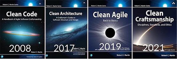
The phrase “clean code” from Uncle Bob’s 2008 book Clean Code has, in some circles, confusingly come to mean “bad code.” Critics argue that clean code is overengineered, is filled with useless abstractions, obscures the flow of control with tiny methods and classes, and leads to poor performance.
I’m going to tease apart the difference between clean code, as described in Uncle Bob’s book, and clean code, a generic term of praise used in engineering contexts for decades. I will debunk the claim that clean code inevitably leads to poor performance, showing exactly when it does and when it doesn’t.
Then we’ll move beyond clean code and talk overhead in general and mixed-language systems which blend together code with different degrees of optimization, and learn why optimizing the wrong thing leads to that defeated and empty feeling.
The Book
Robert C. Martin almost certainly didn’t realize publishing Clean Code in 2008 would lead to so much confusion. The book contains many generic suggestions for writing code, like “use good names,” but also quite a few OOP-specific suggestions. This is because, as Uncle Bob writes in Chapter 1, emphasis his, “Consider this book a description of the Object Mentor School of Clean Code. The techniques and teachings within are the way that we practice our art.”
Wait, what’s Object Mentor? Object Mentor was Uncle Bob’s consulting firm, founded in 1991 and now defunct. They specialized “in object-oriented technologies,” and much of their work was done in Java, which heavily embraces OOP. This is why the Clean Code contains a lot of OOP, not because Uncle Bob thinks only OOP code can be clean, but because it documents the practices of a specific Java shop that he personally ran back in the 1990s and 2000s.
Uncle Bob knew then that his version of Clean Code was only one of many possible takes. Again, in Chapter 1, he wrote, “There are probably as many definitions [of clean code] as there are programmers.” To underscore this, he included several well-known programmer’s definitions of clean code:
Clean code is elegant, efficient and straight-forward.
Bjarne Stroustrup
Clean code is simple and direct.
Grady Booch
Clean code can be read, and enhanced by a developer
other than the original author.
Dave Thomas
Clean code looks like it was written by someone that cares.
Michael Feathers
Nothing about OOP there. These are good generic definitions of “clean code.” We should continue to use “clean code” in this generic sense and not allow it to mean “bad code.” For one reason, clean code was a term long before Uncle Bob’s book.
Usenet
Here are two references to “clean code” from the 1980s:
This is certainly true however, the tendency to write unreadable code is accentuated in Forth because the language itself provides no help whatsoever to aid the programmer in writing clean code.
From net.lang.c 1986
We’ve all come up with a joke about “negative productivity”. You start the day with, say, a thousand lines of crappy code and end the day with 300 lines of clean code–thereby having produced -700 lines of code for the day.
From comp.software-eng 1989
Thought-terminating cliché
Clean code is so divisive in some places online that it’s become a “thought-terminating cliché,” a term used by Robert Jay Lifton in his 1961 book, A Study of “Brainwashing” in China. It’s “thought-terminating” because someone utters the phrase, and the knives instantly come out on both sides — very little can be said above the noise. We should end this petty squabble and lean more on Michael Feathers’ definition: “Clean code looks like it was written by someone who cares.” This means clean code can be written in any language using any methodology.

Casey Muratori
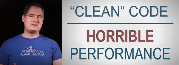
A hot spot in the “clean code is bad code” movement is Casey Muratori’s February 2023 video and blog post, “Clean” Code: Horrible Performance. He uses the phrase “clean code” more than twenty-five times in the post, each dripping with derision and contempt. He presents two versions of a numerical calculation. The first version is OOP, which he says is “clean code,” while the second is a simpler C function with a lookup table. The second version runs 25 times faster than the first after he optimizes it with AVX (x86 SIMD instructions).
Casey’s optimized version is most certainly “clean code,” and he should have said as much in the post. His version solves the problem while being minimal, elegant, and fast. However, perhaps confusingly, the OOP version is also clean code in the same positive sense, but only if the slower speed is acceptable in your use case.
The OOP version is wordier but straight out of an introductory OOP class. It’s the minimal OOP solution: an abstract base class with two virtual methods and four concrete classes that implement those two methods, and that’s it. This is clean code, but heavily into the OOP style.
Performance
Performance is the biggest difference between the two implementations. The optimized version is 25 times faster than the OOP one. Casey puts this performance gap into “iPhone terms,” saying that using the slower version is like forcing yourself to use a really old phone, wiping out “12 years of hardware evolution”.
To him, this means you should never use the OOP version. To me, however, it’s not as definitive. I had a 12-year-old phone, I had one 12 years ago, and it was blazing fast at the time. So I know that level of speed can do useful things. Let’s look at the performance numbers; the cycle counts are from Casey and the other two rows I calculated:
| OOP | AVX | |
|---|---|---|
| Cycles to process one shape | 44.3 cycles | 1.8 cycles |
| Time to process one shape at 3GHz | 14.75 nanoseconds | 0.6 nanoseconds |
| Shapes processed in one millisecond | 67,797 | 1,670,000 |
There are three main reasons why the OOP version is slower than the optimized version:
- The only way the CPU can process large amounts of data efficiently is if the data is stored in a dense linear array. His clean code implementation did not set up memory this way, so it was doomed to poor performance from the start.
- Virtual functions should only be used if the work done inside the virtual function is large compared to the cost of calling the virtual function. His virtual functions were tiny: the largest one contained just two multiplications.
- In the optimized version, he uses AVX (SIMD) instructions. These cannot be used in the OOP version because the code is spread out in different classes; there is no tight inner loop to optimize.
Memory Layout
Memory layout is the most important factor here. In his fast version, the loop iterates over a shape_union *Shapes, which is a dense contiguous array of memory that looks like this:
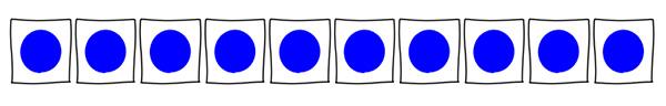
This is what you want. Each blue circle is one of his shape_union objects. The object contains one u32 and two f32 variables, so the size of shape_union is 94 bytes, no extra padding should be needed. In this array, we have 94 bytes related to the first shape followed by 94 bytes related to the second shape, and so on – a dense contiguous array of data. Life is good; the CPU is happy.
In the clean code version, on the other hand, the loop iterates over a shape_base **Shapes. This is an array of pointers to shapes. Here is a first attempt to visualize this version:
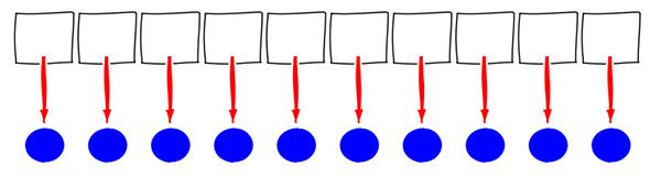
However, this is a very misleading illustration. It implies the shape objects are also neatly organized in memory alongside the main array, but nothing about the type shape_base **Shapes implies or enforces this layout.
Casey didn’t share his allocation code, but most likely, the shape objects were allocated from the heap, which means they could be anywhere in memory, so this is a more accurate depiction of his clean code version:
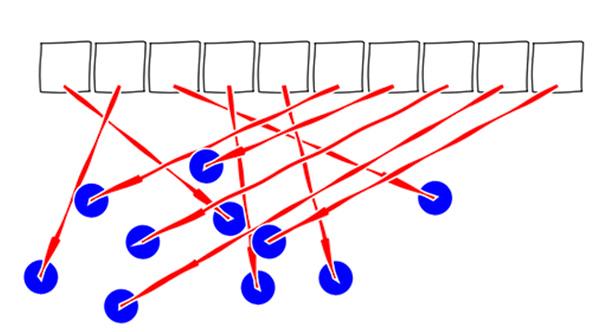
The code is clean, but the data is messy! Objects allocated on the heap are abstractions. For less performance-critical code, we can pretend access to those objects is free, but for low-level performance-critical code, jumping around to random locations in memory is extremely expensive, the CPU hates doing that, so we cannot ignore the cost.
If you think this mess of arrows is an exaggeration because the heap will “probably” give you contiguous allocations, you are in for a nasty surprise. In real applications, the shapes were most likely created at different times, which will scatter their layout. Worse, though, much more scrambling will occur if the array of pointers is sorted, filtered, or altered in any way after creation. The final result is almost certainly going to resemble the above mess.
Nothing we do after this point can undo the damage caused by our scattered memory layout, but let’s look at the virtual functions as well since they are also a problem:
Virtual Functions
    // Square
    virtual f32 Area() {return Side * Side;}
    virtual u32 CornerCount() {return 4;}

    /// Rectangle
    virtual f32 Area() {return Width * Height;}
    virtual u32 CornerCount() {return 4;}

    // Triangle:
    virtual f32 Area() {return 0.5f * Base * Height;}
    virtual u32 CornerCount() {return 3;}

    // Circle:
    virtual f32 Area() {return Pi32 * Radius * Radius;}
    virtual u32 CornerCount() {return 0;}
C++ prides itself on having “zero-cost abstractions,” but virtual functions are not zero-cost. At runtime, the executable has to figure out which concrete method to call using a hidden virtual pointer (vptr) and a hidden virtual table (vtable). It uses these things to “dynamically dispatch” the appropriate method. The overhead of a virtual function call will swamp the work done if the amount of work is too small.
Casey’s virtual functions are close to as small as you can get. The CornerCount() functions contain zero arithmetic operations, they just return a constant. While the Square::Area() and Rectangle::Area() contain one multiplication, and Triangle::Area() and Circle::Area() contain two multiplications. All of them are too tiny to be efficient virtual functions. This flatbed truck is a depiction of a virtual function call whose overhead is larger than the amount of work it’s doing:

A virtual function that's not doing much work.
Flexibility of OOP
If the optimized version was better in every way, the story would end here, just do it the optimized way every time. However the OOP version provides one significant advantage. The way the optimized version gets its dense array of data is this shape_union struct:
enum shape_type : u32
{
    Shape_Square,
    Shape_Rectangle,
    Shape_Triangle,
    Shape_Circle,

    Shape_Count,
};

struct shape_union
{
    shape_type Type;
    f32 Width;
    f32 Height;
};
The shape_union struct dictates that each shape is defined by only a Width and Height, however in the OOP version each concrete shape class contained slightly different data:
| Shape | OOP | AVX |
|---|---|---|
square |
Side |
Width and Height |
rectangle |
Width and Height |
Width and Height |
triangle |
Base and Height |
Width and Height |
rectangle |
Radius |
Width and Height |
Given the speedup obtained, if you only need these four shapes, this slight muddying of the data model is a reasonable price to pay, but it hints at the advantage of the OOP approach: every shape can contain totally different data and implement totally different algorithms. If you are going to add new shapes that require novel data and novel algorithms, only the OOP version can easily handle that. Maybe you need to add polygons with N sides, or curve patches, or a shape swept along a spline, or 3D shapes.
A clean solution has to first and foremost be a solution. If the optimized version 100% solves your problem, then great. But if you are going to need to support a panoply of different shapes, the OOP version has some strong advantages. The ultimate solution might be a mix of the two: maximally fast for simple shapes, but make it possible to support complex shapes. Use the right tool for the job.
Performance Requirements and Analysis
Now let’s dive into performance. Whether the OOP version is fast enough depends entirely on your use case. Imagine two hypothetical games, one complex 3D game that requires processing 1 million shapes per frame, and one simple mobile puzzle game that requires processing 100 shapes per frame:

Hypothetical games: 1 million shapes vs. 100 shapes
The performance of the 3D game:
| OOP | AVX | |
|---|---|---|
| Shapes to process | 1,000,000 | 1,000,000 |
| Time to process 1M shapes | 14.75 milliseconds | 0.6 milliseconds |
| Percent of 60Hz (16.7ms) frame | 88% | 3.6% |
There’s no way we could afford to burn 88% of our frame processing shapes, even if we used a separate thread. But 3.6% sounds reasonable. So this is a huge win for the AVX version. With the OOP version we basically do not have a game, we cannot ship it, but with the AVX version we have a chance. The optimization saves our bacon in this case.
How about the puzzle version:
| OOP | AVX | |
|---|---|---|
| Shapes to process | 100 | 100 |
| Time to process 100 shapes | 1.5 microsecond | 0.06 microseconds (60 nanoseconds) |
| Percent of 60Hz (16.7ms) frame | 0.01% | 0.0004% |
As you’d expect 0.0004% is still 25x faster than 0.01%, but in this case 0.01% is almost certainly fast enough. That means we only burn one-thousandth of the frame to do the shape processing. Let’s look at it another way, how many shapes can we process in a fixed amount of time. I’ll arbitrarily use 1 millisecond as our “budget,” setting budgets is a good practice to get into:
| Shapes in 1 millisecond | OOP | AVX |
|---|---|---|
| 100 | ✅ | ✅ |
| 1,000 | ✅ | ✅ |
| 10,000 | ✅ | ✅ |
| 100,000 | ❌ | ✅ |
| 1,000,000 | ❌ | ✅ |
| 10,000,000 | ❌ | ❌ |
This table summarizes that there’s a range of timescales where the OOP version performs fine, up to 10,000 shapes. But if you need to process 100,000 or 1,000,000 shapes in a millisecond, you absolutely need the AVX version. And then it points out neither can do 10,000,000 shapes in a millisecond.
This is all hypothetical. You need to understand your application and its requirements. Don’t be scared away from using OOP if it meets your needs, but don’t mindlessly use OOP either. Very often a mix of approaches is the best. Many programs start with OOP at a high level, where N is small, but then filters into dense linear arrays when N is large. For example, maybe you have at most 64 characters on screen in your game, so an object per character is fine, but if you are going to draw a million meshes than OOP would be a very bad choice there.
Casey worked at RAD Game Tools for many years. If you are making a “shape processing” library for game developers you might have no idea how many shapes they will process. In that case, providing the optimized version for your users might make more sense. And if you need to support additional shapes, maybe provide both a fast version and a more flexible one: give people a choice.
The Rules
Casey’s Horrible Performance article concludes by railing against “the clean code rules”:
- The rules simply aren’t acceptable.
- The rules are almost all horrible for performance, and you shouldn’t do them.
- The rules need to stop being said unless they are accompanied by a big old asterisk that says your code will get 15 times slower.
He’s completely right and completely wrong at the same time. He’s right that if you need to process hundreds of thousands of shapes in a millisecond, you are totally and utterly hosed if you use the OOP version: it is simply too slow for that. You must use the optimized version in that case. But he’s completely wrong that the OOP version has “horrible performance” for all possible requirements. It can process tens of thousands of shapes per millisecond. If that’s all you need, or if you need fewer, it might be 100% acceptable to you.
OOP, in this case, is like a chainsaw. It’s a tool that works well in many situations but works poorly in other cases. Casey’s shrill insistence that “clean code” performs horribly across the board is similar to a surgeon using a chainsaw to remove a patient’s appendix.
When the surgeon makes a huge mess and kills the patient, he stands up on the blood-spattered operating room table and gives a passionate speech about how chainsaws should never be used for any purpose ever, by anyone. Meanwhile, millions of people worldwide productively use chainsaws every day, just like millions of developers successfully use OOP. A chainsaw has a lot of uses, but performing appendectomies is not one of them, so don’t use it for that, and don’t use OOP where you need maximally efficient inner loops. This chart summarizes our findings:
| OOP | Okay? | Chainsaw | Okay? |
|---|---|---|---|
| Nanoseconds | ❌ | Abdominal Surgery | ❌ |
| Microseconds | ✅ | Tree Limb | ✅ |
| Milliseconds | ✅ | Small Tree | ✅ |
| Seconds | ✅ | Large Tree | ✅ |
Even more overhead
The previous table showed that the “clean code overhead” was 42.5 cycles, 14.5 nanoseconds on a 3GHz machine. But let’s go crazy with this next table. Let’s assume the overhead of our clean code, or whatever methodology we use, is 100 nanoseconds. A huge amount of overhead, 300 times longer than a clock tick. This might be even slower than an interpreted language like Python or Javascript, but it doesn’t matter what the source of the overhead is. This is the damage that 100 nanoseconds will do:
| Duration of Loop Body | Amount of Overhead | Descriptive Term |
|---|---|---|
| 2 nanoseconds | 5000% | Crazy huge |
| 2 microseconds | 5% | Relatively small |
| 2 milliseconds | 0.005% | Impossible to measure |
| 2 seconds | 0.000005% | Impossible to measure |
The impact of 100 nanoseconds disappears quickly as we go lower in the table because this chart depicts nine orders of magnitude of durations. To state the obvious, two seconds are 1,000,000,000 times longer than two nanoseconds. Well, duh, but our hunter-gatherer brains weren’t built to think about durations of time that span nine orders of magnitude. If you work mostly in one of these timescales, it’s easy to forget the others even exist, let alone be facile in thinking about them.
The above chart gets at the heart of every disagreement about the performance implications of clean code, which I’ve seen ricocheting around X and YouTube for the last year. Inevitably, one person is thinking about the first row while the other person is thinking about one of the other rows, but neither discloses the time scale they are dealing with, and hilarity ensues.
Here’s the same chart but to make it more relatable we’ll use a little story. Imagine you are packing your bags for a trip, and it takes you 50 minutes to pack your bags. Here’s the amount of overhead, the amount of time spent packing, relative to the length of the trip:
| Trip Duration | Natural Units | Amount of Overhead |
|---|---|---|
| 1 minute | 1 minute | 5000% |
| 1,000 minutes | 16.57 hours | 5% |
| 1 million minutes | 1.9 years | 0.005% |
| 1 billion minutes | 1903 years | 0.000005% |
Hopefully it’s clear why 50 minutes of overhead has negligible impact on a trip that lasts for 1903 years! This is the same impact 100ns of overhead has if the unit of work is two seconds.
The concept of “overhead” is common to many disciplines; much skull time has been devoted to thinking about it. People worry about overhead in fields as diverse as operations research, supply chain management, systems engineering, chemical engineering, etc. It goes like this: there’s some work we want to do, but we can’t do it all at once, so we divide that work into batches. However, there is some overhead related to each batch. Given all this, how big should the batches be?
How are the size of these important resources chosen:
- Disk blocks
- Network packets
- Virtual memory pages
- Caches and cache lines
- I/O buffers
How about shipping containers, the ones carried by ships, trucks and trains, not Docker containers. In all cases, there’s overhead associated with each unit of work, so we carefully size the unit of work relative to the overhead to strike a good balance between efficiency, latency, and any other concerns.
How big should bites of your sandwich be? If you chewed and swallowed after every cubic millimeter of rye bread, you’d exhibit horrible eating performance, so instead, we choose a bite-size that’s, well, bite-sized. If you only need to do 1.8 nanoseconds of real work, you cannot tolerate essentially any overhead, but if you are doing even a microsecond’s worth of work at a time, those bites are a thousand times bigger, so the overhead is proportionally far less.
Video games
Casey worked at RAD Game Tools, which sells libraries used in “thousands and thousands” of shipping games. A hyper-fixation on performance can be warranted inside game engines or game libraries. But engines and libraries stand in contrast to “the game code,” which is often not performance-critical. Instead of running millions of times, game code might run just once at one specific point in the game.

Rockstar expects to release GTA 6 in Fall 2025
Rockstar’s Advanced Game Engine (RAGE) has been used to power ten popular games over the last two decades, including the hotly anticipated Grand Theft Auto VI that’s been under development for years, due out in 2025. However, most of the 2,000+ developers making GTA 6 are not working on the engine; they are working on the code, art, or design related to the missions the player will advance through in the single-player campaign. Since there is so much game code to write, and it’s generally not performance-critical, developers often move the game code to a scripting language.

Guitar Hero franchise grossed $2 billion within four years of release.
I was the lead programmer on the original Guitar Hero for PlayStation 2 in 2005, and that’s how we did it. About two-thirds of the game was written in C++ for speed, but one-third was in a proprietary scripting language. Eric Malafeew, the Chief Architect and Engineering Lead, invented the language and tenderly nurtured its development. It looked similar to Lisp and was a simple text file anyone could edit without the need to recompile the game.
For instance, the C++ code would emit an event when the song ended, and a script hook would trigger animations and sounds to explode the track. This way, designers and artists could edit the script without a programmer’s involvement. This flexibility was critical to iterating quickly: the entire game was developed in nine months, start to finish. Take that, Rockstar.
You can find similar pairings of fast and slow languages everywhere in the modern computing landscape, far beyond games. For instance, your web browser is probably written in C++, but almost every website you visit is powered by Javascript, a much slower language. The V8 Javascript Engine alone has nearly two million lines of C++, but it can run scripts from hundreds of millions of different websites, none of which need to have a C++ programmer on staff. This division of labor allowed millions of people to create websites: if every website had to be written in C++, the web would be a very different place.
Python
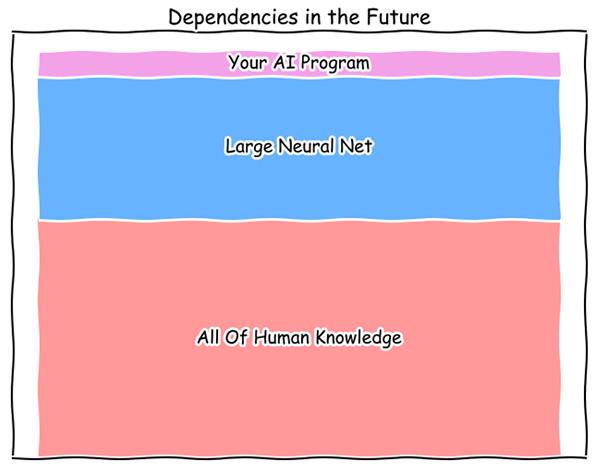
The Python ecosystem is another place where a mix of programming languages, and thus differing degrees of overhead, is incredibly effective. Below are some possible dependencies for a machine-learning application written in Python.
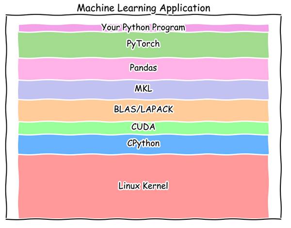
The dependencies of a Machine Learning application written in Python.
Combined, these dependencies contain millions of lines of C/C++, Rust, and even Fortran code, much of which is heavily optimized for speed. The existence of layers written in different languages is an amazingly effective and productive arrangement. Splitting responsibilities into layers allows large numbers of people to tackle ambitious problem domains concurrently because they focus their job, maybe their entire career, on one particular layer. I admire and respect the people working on every dependency in this chart, all layers are important.
Mixture of Optimization Levels
Imagine a world where every bit of code everywhere had to be hyper-optimized. Everything had to be written in C or assembly and was carefully engineered for maximum speed. Everything would be super fast! The chart below depicts that world. The Y-axis is the log of the amount of overhead, while the X-axis is the log of the number of operations performed with that amount of overhead. This chart shows us doing quadrillions of computations, and the overhead is never more than a nanosecond:
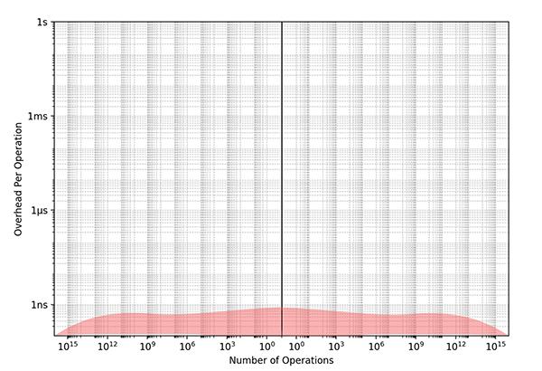
Everything is maximally optimized.
The above might be possible for a small high-performance library, such as a core neural network kernel, but it’s impossible to achieve this level of uniform optimization for a sprawling codebase; it would be way too much effort. Instead consider a program written in a high-level language like Python without optimized libraries. Everything is in “pure Python,” so the overhead of every operation is large. We do far fewer operations because it just wouldn’t be tractable to do zillions of operations in pure Python:
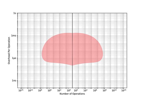
Program written in Pure-python or any "slow" language.
The next plot is what’s common in the real-world for large systems, which is generally what you want. An application was written in Python or some other high-level language using optimized lower-level libraries. Since the X-axis is log, there are many orders of magnitude more fast operations even though it’s only a bit wider:
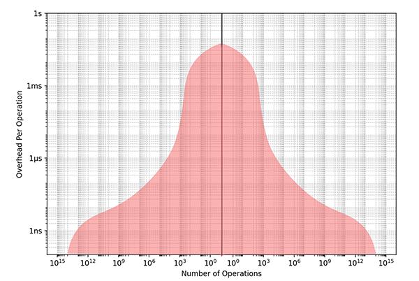
A program written with a blend of languages and styles.
This is a healthy system. Wherever needed, we implement computations in faster languages or with more optimized techniques, but we don’t needlessly optimize the whole world. We keep the higher-level code accessible to a wider audience of software engineers, where changes can be made quickly. We constantly re-evaluate slower code and promote it to faster code whenever needed, whether by ourselves or by adopting a library someone else carefully optimized for us.
Diversity in the Time Domain
There’s tremendous diversity in the software industry, in the same way there is in the construction industry. Construction workers build sheds, houses, townhouses, apartment buildings, shopping malls, gleaming office towers, stadiums, bridges, nuclear power plants, and launchpads for rockets to Mars. All of these things are useful in their own way.
In software, the diversity is less visible. To the untrained eye, all programmers do roughly the same thing: typing on our keyboards and staring at the screen. But the software we are developing does vary drastically. Here are some of the projects I’ve personally worked on over the last thirty years and the time scales that were involved:
| Problem Domain | Update Frequency | Cycle time |
|---|---|---|
| LED Ceiling Tracker | 3000Hz | 300us |
| Haptic Device | 1000Hz | 1ms |
| Graphics (Console game) | 60Hz | 16.7ms |
| Graphics (VR) | 120Hz | 8.3ms |
| Responsive Button Press | Once | 100ms |
| Natural language ML task | Continually | 10 seconds |
| Point cloud and spherical image processor | Once a week | Days |
Again, this is nine orders of magnitude of cycle times. I once talked to a woman on a plane who was a video editor. She saw me writing code and asked about it. I asked her about video editing. We agreed that video editing was very technical and complicated, but that software was markedly different because there was no bottom.
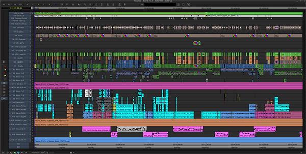
Timeline for one reel of Mission: Impossible - Rogue Nation (2015)
Lets see how deep software goes. If you want to read about the AVX instructions that Casey used in his fast version, crack open Intel’s 5,000-page PDF on the x86 instruction set, a little nighttime reading:
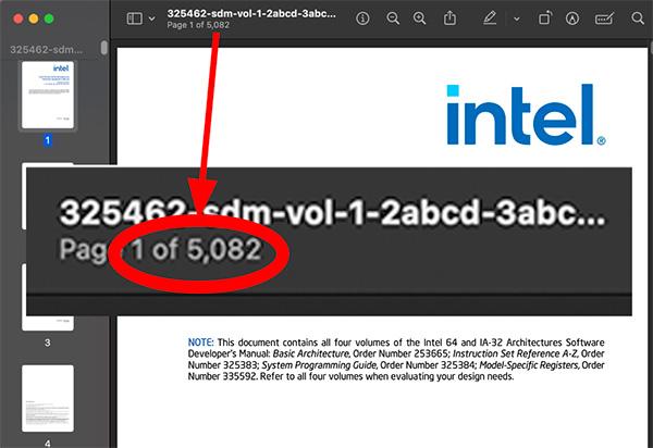
Read about AVX in Intel's x86 instruction set manual.
And when you’re done with that, start reading about transistors, fabrication design, photolithography, etching, and doping. Then, move on to how we mine the raw materials.
In the other direction, upwards, if you use AWS or any cloud vendor, they have billions of lines of code that run on hundreds of thousands of computers, each one of which has all the full complexity of a single machine running regular software. Meanwhile, if you are writing a large application that runs in the cloud, you are piling things higher still, building on top of the whole sordid affair.
The idea of cooperating layers at different levels of abstraction predates Computer Science — it’s embedded in reality itself. There are hundreds of academic fields at a large University, but here are eight of them roughly arranged into layers:
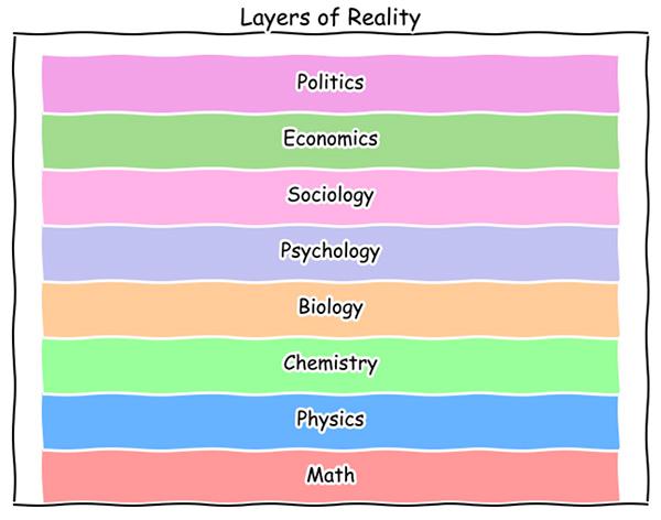
Layers of academic fields studying reality.
As with software, a higher layer can reach way down to any lower dependency: any of these fields, except perhaps for Politics, can do Math. The lowest levels here, Math and Physics, have a reputation for being conceptually difficult and technically challenging, like working on a game engine or the Linux kernel, but interesting, important, and difficult work is done in all of these layers.
Natural Language Programming
As we speak, Artificial Intelligence is rapidly reshaping the computing landscape. It will allow people to “program” in natural languages, like English or any human language, potentially expanding who can be a programmer to the entire world. While all the traditional software layers will still exist underneath, the conceptual model of people writing “code” in the future might be something like this:
Conceptual model for natural language programming.
If you cringe at how much computation a single line of Python can invoke, you’ll faint when you see how much compute and energy these large neural networks will burn. The total energy available worldwide will be the limiting factor when everyone can expend trillions of CPU cycles just asking for the weather. As you’d expect, though, virtually all of those cycles will be running in hyper-optimized code, eventually in hyper-optimized hardware as well.
Each layer is critically important in a tall stack of dependencies. Imagine the grand opening of a Las Vegas hotel with gleaming marble floors, oceans of high-tech gaming machines, and a fancy theater with an aging pop star in residence. Now, imagine every toilet in the building is overflowing. We need every layer to work efficiently and be free of security vulnerabilities. Achieving that will take tremendous effort forever.

Humans are tool makers as much as tool users.
However, Object-Oriented Programming isn’t a layer; it’s a tool. When I was discussing Casey’s optimization post on X, Uncle Bob himself chimed into our thread, saying don’t use clean code if it’s too slow for your needs. He wrote, “It is generally true that any tool you use must be worth using. The benefit must exceed the cost.”
Functional Programming
The famous SICP uses Scheme, a Lisp variant to teach FP.
Years after writing Clean Code, Uncle Bob had an epiphany reading the famous MIT book Structure and Interpretation of Computer Programs (SICP) by Harold Abelson, Gerald Sussman, and his wife, Julie Sussman. The book uses Scheme, a variant of Lisp, as its teaching language. Uncle Bob was so taken in by the book he’s spent much of the last decade programming in Clojure, a Lisp dialect that runs on the JVM. Conveniently, any JVM language can interoperate with Java, his previous go-to language.
Uncle Bob hasn’t denounced OOP but says FP and OOP (and even procedural) are valid approaches to writing software. He says use whichever makes sense for the problem you are trying to solve, a sane and pragmatic stance that doesn’t require slagging someone’s life’s work.
Physical Bits
Software development is a game of intense cooperation between you and millions of strangers you will never meet. We interface through a giant codebase we’ve been building for eighty years. There is room for everyone, whether you join late and write “code” in English or have spent decades perfecting hand-tuning your assembly one instruction at a time, we need it all.

Frederick P. Brooks Jr. Computer Science Building at UNC-Chapel Hill.
When I worked as a Research Engineer at UNC-Chapel Hill, Fred Brooks randomly popped into meetings and offered sage advice. He was a kind and insightful person. In The Mythical Man-Month, he wrote, “The programmer, like the poet, works only slightly removed from pure thought-stuff. He builds his castles in the air, from air, creating by exertion of the imagination.”
Of course, the Turing Award winner was right, but there is more. We first build castles in the air, in our heads, but then we encode them into bits. Not ethereal abstract bits, not platonic bits, but real physical bits: the orientation of magnetic domains on a hard drive, electrical charges in floating-gate transistors in an SSD, tiny capacitors in RAM, optical pulses on a fiber optic cable.
At any given time, like right now, you could combine every physical bit of software on the planet, place them end-to-end, in a dense contiguous array, and then interpret the result as a single gigantic integer. One number representing the sum total of all software humans have created. This leads to two intriguing questions. How large will this number ultimately grow? And what was the previous high score?
YouTube Video